Value has been recognised as one of the most important factors for equities at least since the pioneering work by Fama and McBeth (1973). In equities, the ratio of book-to-market value has traditionally been used as a proxy for the value factor.
Natural as this choice is for this asset class, it is difficult to translate the concept of value to the fixed-income domain, and for this reason Fama and French (1993) argued that value does not apply to fixed-income instruments in general, and to Treasury bonds in particular. This seems to be at odds with recent literature, which claims to have found value (and momentum) ‘everywhere’.
The ‘problem with value in bonds’ is rendered more acute by the rather ad hoc definitions of value used for fixed-income instruments. For instance, Asness, Moskowitz and Pedersen (2013) defined value for bonds as the (negative of the) five-year bond returns – a choice motivated by the observation that in equities this difference in returns is found to be positively correlated with the book-to-market ratio.
The factor thus defined may well predict future bond returns, but its interpretation as ‘value’ seems at least a stretch, and one, if not two, steps removed from the true latent underlying factor. At best, it plays the role of a proxy, and as a result, labelling the chosen measure as value becomes rather arbitrary.
In this article, we provide what we think is a more intuitively satisfactory definition of value in US Treasury bonds, and we show that the value quantity we define has very strong predictive power of future cross-sectional Treasury returns.
More precisely, we identify ‘cheap’ (‘valuable’) and ‘expensive’ bonds using a dynamic Gaussian term structure model, and show that a systematic, no-peek-ahead strategy of investing in the cheap bonds and shorting the expensive ones has a strongly positive Sharpe ratio.
Our results are so robust that, before and after adjusting for duration exposure, the strategy we propose has positive Sharpe ratios for 14 of the 15 three-year periods from 1975 to 2017, a Sharpe ratio which is statistically significantly different from zero at the 99.9% confidence level in 13 of the 15 three-year sub-periods, and an average Sharpe ratio (before transaction costs) above 1.
Dataset
The data used for the study is made up of the daily close-of-business day prices of 1,562 US Treasury coupon bonds over the period 27 December 1973 to 29 June 2018. All these bonds are non-callable, non-puttable and non-inflation linked. We also excluded prices of individual bonds that were deemed to be erroneous from the dataset.
This was determined by setting a threshold in standard deviations for the price changes, and then excluding those bonds whose price move exceeded the threshold while the other bonds in the universe for that day did not show a similar move. We stress that this culling procedure is conservative because spurious spikes would generate fictitious profits: we, therefore, prefer to miss a true sharp price deviation/reversal than to include a fake one.
Interest rate model
The affine model we employ can be defined in the physical (P) and risk-neutral (Q) measures. Starting from the P measure, it can be written as:
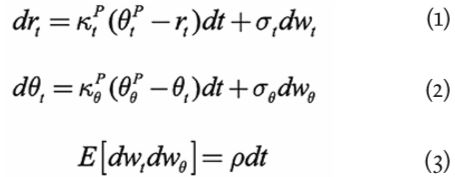


The model can be interpreted as describing the actions of the monetary authorities who respond to deviations of the inflation and/or output gap from their desired target levels by adjusting the Fed funds rate (in our model, the ‘short rate’) towards the long-term NAIRU-compatible nominal rate (the ultimate reversion level ); they do so, however, with a degree of urgency (‘aggressiveness’) that depends on the economic conditions of the moment; the adjustment is therefore achieved by letting the short rate revert to a time-dependent reversion level, which in turn reverts towards the unchanging NAIRU-compatible long-term nominal rate,.
In moving from the physical to the risk-neutral measure we assume that investors only seek compensation for level risk (see, in this respect, Cochrane and Piazzesi [2005]; Adrian, Crump and Moench [2010]), and therefore modify the P-measure dynamics in equation (2) as:

In general, the market price of risk could depend on both state variables. We make the assumptions:
• That the slope of the yield curve accounts for the degree of predictability associated with the business-cycle variation of risk aversion; and
• That the additional predictability afforded by the new-generation return- predicting factors (eg, Rebonato and Hatano [2018]; Cieslak and Povala [2010]) is due to deviations from fundamentals, and not to non-level rewarded risk factors.
Since our approach tries to capture precisely these deviations from fundamentals, we do not add other contributions to the market price of risk other than its business cycle/slope-related component. If we want to retain the essentially affine formulation, the market price of risk must display, at most, an affine dependence on the state variables. In other words, it must have the following form:


We assume = 0 (see Duffee [2002] for a justification of this choice). Cochrane and Piazzesi (2005), as well as Adrian, Crump and Moench (2013) document that investors only seek compensation for bearing level risk. Given the high reversion speed of the short rate, we therefore impose the condition that only the uncertainty about the reversion level,, should attract a risk premium. This implies that the process for the short rate should be the same under P and Q. Finally, we require that the market price of risk should depend on the slope of the yield curve (Fama and Bliss [1987]; Campbell and Shiller [1991]). More details on the model formulation, the connection between the real-world and the pricing measure and the model calibration can be found in Rebonato, Maeso and Martellini (2019).
The model prices of the coupon bonds are calculated as:


where denotes the the time-t price of a T-maturity coupon-bearing bond with N coupons still to pay, signifies the time-t price of a discount bond of maturity , and the cash flows include both the coupons and the final repayment at maturity.
Creating the strategy signal
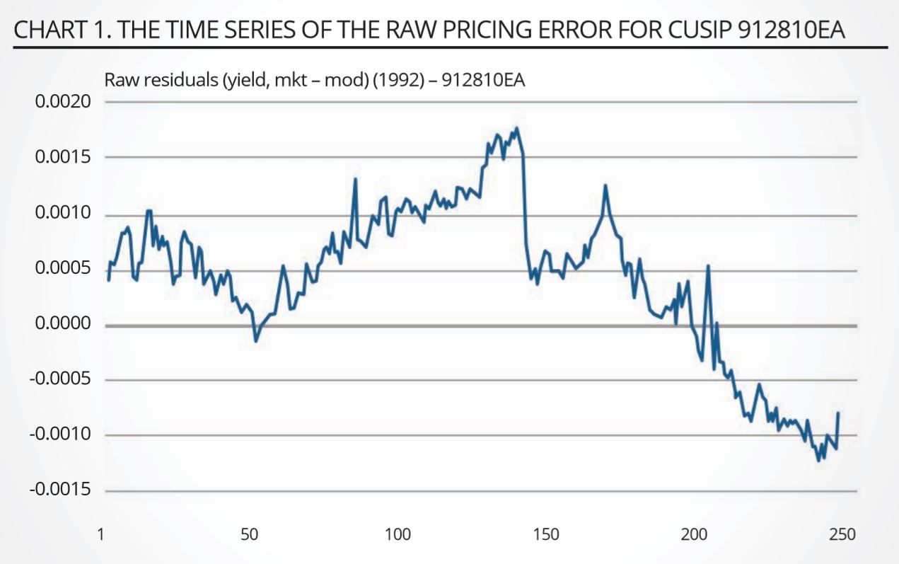
After the calibration procedure has been carried out, for each bond we have a time series of pricing errors. One such series for a particular Treasury bond is shown in chart 1. To establish a trading strategy, we create a trading signal by setting the notional of the position in each bond to be proportional to the strength of the signal for that bond on that day.
Source: EDHEC Risk-Institute
For each bond, the trading signal is formed by taking the difference between a slow-moving average and an adjusted fast-moving average of price errors. The adjusted fast-moving average is obtained by summing the last nshort price errors, and dividing the sum by nlong, rather than nshort, where nlong and nshort are the number of price errors in the long and short sum, respectively.
We use a slow-moving average, rather than the zero level, for the pricing errors because some bonds (perhaps for liquidity or other reasons) may have an unconditional average price error different from zero. The reason for using an adjusted fast-moving average, that is, for dividing the short sum by nlong, rather than nshort, is to make the signal more stable and to filter out high frequency (quickly reversed) price errors, clearly visible in the time series displayed in chart 1, that can lead to overtrading.
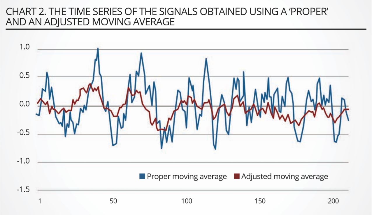
The differences in signal using a proper and an adjusted moving average are shown in chart 2, which was obtained using a random walk to obtain the price errors, nlong = 20 and nshort = 5. It is clear that the adjusted signal retains the salient trends, but removes the high-frequency fluctuations, which is exactly what we wanted to achieve. We took the number of days in the slow-moving average as equal to 22 business days (corresponding to roughly one month), and the number of days in the fast-moving average ranging from one to five business days (with the last choice corresponding to roughly one week).
Source: EDHEC Risk-Institute
We stress that the results we report in the following section were not obtained for any optimised combination of days in the fast- and slow-moving averages: as the round numbers (22 and one or five) and their simple interpretation (one month and one day/one week) indicate, we did not engage in a datamining exercise of optimisation. The same applies to the cut-off maturities (two and 15 years).
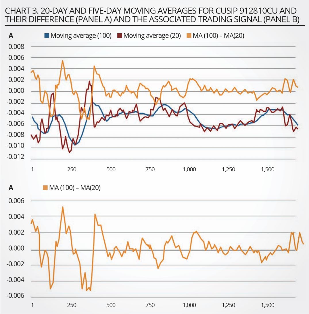
Typical patterns for the two moving averages and the resulting signal are shown in chart 3. As this shows, the trading signals tend to display mean-reverting behaviour, with reversion speeds implying half-lives of several weeks to a few months. This observation is important, because it suggests that the signal is practically exploitable, in that it neither requires excessively long strategies, nor overly frequent rebalancing.
Source: EDHEC Risk-Institute
On any given day, our strategy will consist of long positions in cheap bonds and short positions in expensive bonds. The resulting portfolio will not have a systematic long or short bias but, on any given day, it will not have exactly zero cost, nor will it be exactly duration-neutral.
Because yields fell considerably over the period under study, we control for a possible residual duration exposure in our portfolio by calculating the net portfolio duration, and by subtracting the hypothetical profit (or loss) that a portfolio with that residual duration would make given the change in average yield from one day to the next. We note that subtracting the duration exposure this way would flatter the results from long positions, and penalise short positions, because achieving physical (as opposed to virtual) immunisation requires selling an actual bond.
Over the period under study, Treasuries have commanded an unconditional positive risk premium, and therefore physical hedging requires paying, rather than receiving, this premium. (To give an idea of the size of the effect, the magnitude of the unconditional risk premium for the 10-year point is over 200 basis points per annum.)
To compensate for this, we increase the funding cost by an amount required to ensure zero realised return in each three-year period for a virtually duration-neutralised equal-weight long bond portfolio. We funded the difference between the proceeds from the short sales and the cost of the long positions by borrowing or lending at the Treasury Bill rate. Finally, we reinvested all coupons received in the same bond from which they originated.
Profitability of the strategy
We carried out our analysis of the results by splitting the data into 15 blocks of three years (the last block is slightly shorter than three years). We have no return results for the first few days of each three-year block because of the need to build the moving average needed for the signal.
Source: EDHEC Risk-Institute
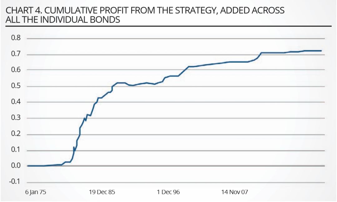
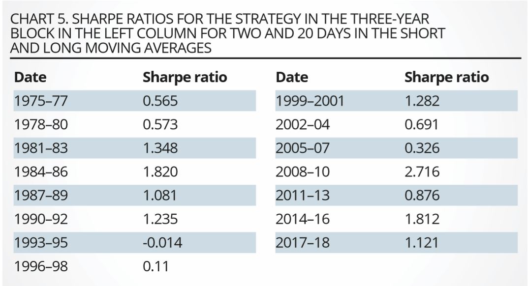
On any given day, the overall strategy will in general consist of long and short positions in different bonds. Chart 4 shows the cumulative profits for the duration-corrected strategy. The ratio of the strategy returns and volatility – ie, the Sharpe ratio of the funded, duration-neutralised strategy – is shown in tabular form in chart 5.
Source: EDHEC Risk-Institute
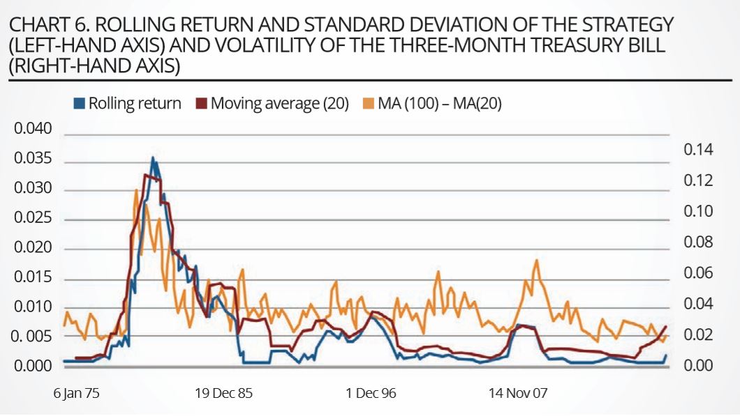
We stress that the Sharpe ratio is positive in 14 of the 15 three-year blocks, is often very high, is never significantly negative, and is significantly greater than zero at the 99.9% confidence level in 12 of the 15 blocks. It is clear that the Sharpe ratio of the strategy is very high, but also that it has tended to decline over time. By far the most interesting observation, however, is the high correlation (75%) between the short-rate volatility (either as obtained from the fitting of the model, or as estimated statistically as the volatility of the three-month Treasury Bill rate) and the profitability of the strategy, displayed in chart 6.
Source: EDHEC Risk-Institute
We also note that the strategy tends to produce high returns – but not necessarily high Sharpe ratios – when the market volatility is high; in these periods the volatility of the strategy is also high, and therefore the Sharpe ratios do not display this link with the market volatility. This finding is significant because it suggests a clear indication of the origin of the profitability of the strategy.
Our results can, in fact, be reconciled with the findings by Hu, Pan and Wang (2013), who establish a link between price errors (‘noise’ in their terminology, page 2341) for Treasury bonds and a general decrease in market liquidity. The explanation they offer is that the greater the decrease in liquidity, the greater the difficulty encountered by pseudo-arbitrageurs in carrying out the trades that should bring Treasury prices in line with fundamentals.
To the extent that an increase in volatility can be associated with a decrease in market liquidity, the findings of our study are consistent with the interpretation in Hu, Pan and Wang (2013), and provide a rationale for the source of profitability of our strategy. And if high returns are indeed achieved in periods of high market volatility, it is not surprising that in these periods the volatility of the strategy should also be high, as the deviations from fundamentals may well increase (giving rise to temporary losses) before eventually decreasing towards their reversion level.
Long-only analysis
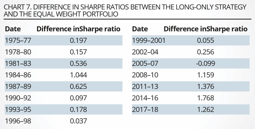
We also explored a long-only version of our strategy by only investing in those bonds that, according to the model, were underpriced (cheap), and investing an equal amount in all the bonds in the universe (we call this the equal-weight portfolio). The market and strategy portfolios were sized to require the same outlay of cash, and both versions of the strategy were funded and duration- neutralised as explained in the previous section. We report the results in chart 7.
Source: EDHEC Risk-Institute
As mentioned, the funding rate was adjusted in each three-year block so as to give a zero Sharpe ratio for the long-only equal-weight portfolio. In terms of Sharpe ratio, the long-only strategy outperforms the market portfolio in 14 of the 15 three-year periods. The average Sharpe ratio for the strategy is significantly higher than that of the long-always strategy at the 99% confidence level.
Although from the theoretical point of view, these results do not add much to the results shown in the ‘Profitability of the strategy’ section, they are very important for the practical applicability of the strategy for many institutional investors, who often have long-only constraints.
Conclusion
In this article, we have proposed a definition of value in Treasury bonds that, we believe, displays more clearly the features intuitively associated with the term ‘value’ than what has recently been offered in the literature. In our definition, value is the difference between the market price of a Treasury bond and its theoretical price, with the latter determined by a financially motivated dynamic Gaussian term structure model.
Using this definition of value, we construct long/ short self-financing portfolios that load positively/ negatively on our value factor. After controlling for residual duration exposure, we show that the portfolios thus constructed consistently earn a very attractive Sharpe ratio (average Sharpe ratio of 1.03, with a positive Sharpe ratio in 14 of the 15 three-year periods in our dataset). The Sharpe ratio of a long-only version of the strategy outperforms that of an equally weighted long portfolio by 0.822.
We have shown that the profitability of the strategy is closely linked to the volatility of the three-month Treasury Bill. We can explain this finding if we establish a link between higher market volatility and poorer market liquidity. In this account of our finding, in periods of market turmoil (of high volatility), less arbitrage capital is forthcoming to bring prices back to fundamentals, and pricing errors temporarily appear. As market conditions revert to normal, the pricing errors are arbitraged away toward zero.
Our study did not try to account for trading costs, but, given the size of the Sharpe ratio, it appears unlikely that trading costs in the extremely liquid Treasury market could wipe out, or significantly reduce, the profitability of the strategy.
Finally, it would be interesting to undertake a systematic study of the timing of the profitability of our strategy, compared with the returns from a diversified US equity index, or from the various equity factors that have been identified in the literature. We leave this as a possible future development.
Jean-Michel Maeso is senior quantitative researcher at EDHEC Risk Institute, Lionel Martellini is Professor of Finance at EDHEC Business School and Director of EDHEC-Risk Institute and Riccardo Rebonato is Professor of Finance at EDHEC-Risk Institute.
This article first appeared in the Q2 2020 edition of Beyond Beta, the world’s only smart beta publication. To receive a full copy, click here.


